 阿源的知识库
聚类算法
8. 聚类算法原理
kmeans
优势: 简单,快速,适合常规数据集 K值难确定 劣势: 复杂度与样本呈线性关系 很难发现任意形状的簇
db聚类
优势: 不需要指定簇个数 擅长找到离群点(检测任务) 可以发现任意形状的簇 两个参数就够了
劣势
高维数据有些困难(可以做降维) Sklearn中效率很慢(数据削减策略) 参数难以选择(参数对结果的影响非常
9. Kmeans代码实现
python
10. 聚类算法实验分析
Kmeans
python
import numpy as np
import os
%matplotlib inline
import matplotlib
import matplotlib.pyplot as plt
plt.rcParams['axes.labelsize'] = 14
plt.rcParams['xtick.labelsize'] = 12
plt.rcParams['ytick.labelsize'] = 12
import warnings
warnings.filterwarnings('ignore')
np.random.seed(42)

from sklearn.datasets import make_blobs

blob_centers = np.array(
    [[0.2,2.3],
     [-1.5,2.3],
     [-2.8,1.8],
     [-2.8,2.8],
     [-2.8,1.3]])

blob_std =np.array([0.4,0.3,0.1,0.1,0.1])
X,y = make_blobs(n_samples=2000,centers=blob_centers,
                     cluster_std = blob_std,random_state=7)

def plot_clusters(X, y=None):
    plt.scatter(X[:, 0], X[:, 1], c=y, s=1)
    plt.xlabel("$x_1$", fontsize=14)
    plt.ylabel("$x_2$", fontsize=14, rotation=0)
plt.figure(figsize=(8, 4))
plot_clusters(X)
plt.show()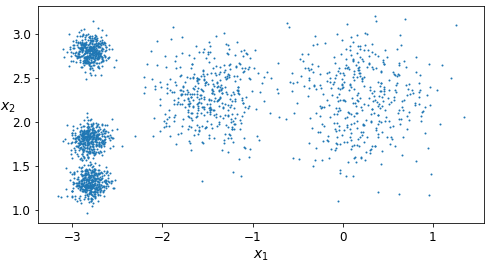
决策边界
python
from sklearn.cluster import KMeans
k = 5
kmeans = KMeans(n_clusters = k,random_state=42)
y_pred =  kmeans.fit_predict(X)

# fit_predict(X)与kmeans.labels_ 得到预测结果是一致的
# 分类标签
y_pred
kmeans.labels_
array([4, 0, 1, ..., 2, 1, 0])
# 中心点
kmeans.cluster_centers_
array([[-2.80389616,  1.80117999],
       [ 0.20876306,  2.25551336],
       [-2.79290307,  2.79641063],
       [-1.46679593,  2.28585348],
       [-2.80037642,  1.30082566]])
python
X_new = np.array([[0,2],[3,2],[-3,3],[-3,2.5]])
kmeans.predict(X_new)
array([1, 1, 2, 2])

kmeans.transform(X_new)
array([[2.81093633, 0.32995317, 2.9042344 , 1.49439034, 2.88633901],
       [5.80730058, 2.80290755, 5.84739223, 4.4759332 , 5.84236351],
       [1.21475352, 3.29399768, 0.29040966, 1.69136631, 1.71086031],
       [0.72581411, 3.21806371, 0.36159148, 1.54808703, 1.21567622]])

def plot_data(X):
    plt.plot(X[:, 0], X[:, 1], 'k.', markersize=2)

def plot_centroids(centroids, weights=None, circle_color='w', cross_color='k'):
    if weights is not None:
        centroids = centroids[weights > weights.max() / 10]
    plt.scatter(centroids[:, 0], centroids[:, 1],
                marker='o', s=30, linewidths=8,
                color=circle_color, zorder=10, alpha=0.9)
    plt.scatter(centroids[:, 0], centroids[:, 1],
                marker='x', s=50, linewidths=50,
                color=cross_color, zorder=11, alpha=1)

def plot_decision_boundaries(clusterer, X, resolution=1000, show_centroids=True,
                             show_xlabels=True, show_ylabels=True):
    mins = X.min(axis=0) - 0.1
    maxs = X.max(axis=0) + 0.1
    xx, yy = np.meshgrid(np.linspace(mins[0], maxs[0], resolution),
                         np.linspace(mins[1], maxs[1], resolution))
    Z = clusterer.predict(np.c_[xx.ravel(), yy.ravel()])
    Z = Z.reshape(xx.shape)

    plt.contourf(Z, extent=(mins[0], maxs[0], mins[1], maxs[1]),
                cmap="Pastel2")
    plt.contour(Z, extent=(mins[0], maxs[0], mins[1], maxs[1]),
                linewidths=1, colors='k')
    plot_data(X)
    if show_centroids:
        plot_centroids(clusterer.cluster_centers_)

    if show_xlabels:
        plt.xlabel("$x_1$", fontsize=14)
    else:
        plt.tick_params(labelbottom='off')
    if show_ylabels:
        plt.ylabel("$x_2$", fontsize=14, rotation=0)
    else:
        plt.tick_params(labelleft='off')
python
plt.figure(figsize=(8, 4))
plot_decision_boundaries(kmeans, X)
plt.show()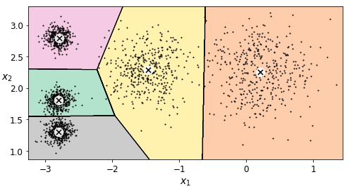
算法流程
python
# 展示了迭代的过程
kmeans_iter1 = KMeans(n_clusters = 5,init = 'random',n_init = 1,max_iter=1,random_state=1)
kmeans_iter2 = KMeans(n_clusters = 5,init = 'random',n_init = 1,max_iter=2,random_state=1)
kmeans_iter3 = KMeans(n_clusters = 5,init = 'random',n_init = 1,max_iter=3,random_state=1)

kmeans_iter1.fit(X)
kmeans_iter2.fit(X)
kmeans_iter3.fit(X)

plt.figure(figsize=(12,8))
plt.subplot(321)
plot_data(X)
plot_centroids(kmeans_iter1.cluster_centers_, circle_color='r', cross_color='k')
plt.title('Update cluster_centers')

plt.subplot(322)
plot_decision_boundaries(kmeans_iter1, X,show_xlabels=False, show_ylabels=False)
plt.title('Label')

plt.subplot(323)
plot_decision_boundaries(kmeans_iter1, X,show_xlabels=False, show_ylabels=False)
plot_centroids(kmeans_iter2.cluster_centers_,)

plt.subplot(324)
plot_decision_boundaries(kmeans_iter2, X,show_xlabels=False, show_ylabels=False)

plt.subplot(325)
plot_decision_boundaries(kmeans_iter2, X,show_xlabels=False, show_ylabels=False)
plot_centroids(kmeans_iter3.cluster_centers_,)

plt.subplot(326)
plot_decision_boundaries(kmeans_iter3, X,show_xlabels=False, show_ylabels=False)

plt.show()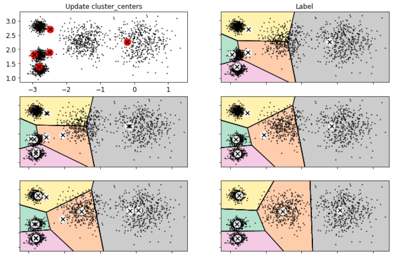
不稳定的结果
初始的随机种子不一样,得到的结果也不同
python
def plot_clusterer_comparison(c1,c2,X):
    c1.fit(X)
    c2.fit(X)

    plt.figure(figsize=(12,4))
    plt.subplot(121)
    plot_decision_boundaries(c1,X)
    plt.subplot(122)
    plot_decision_boundaries(c2,X)

c1 = KMeans(n_clusters = 5,init='random',n_init = 1,random_state=11) # 随机种子 初始中心点
c2 = KMeans(n_clusters = 5,init='random',n_init = 1,random_state=19)
plot_clusterer_comparison(c1,c2,X)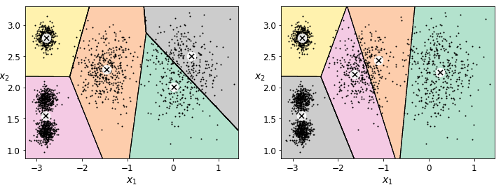
评估方法
python
# Inertia指标:每个样本与其质心的距离

kmeans.inertia_ # 希望越小越好
211.5985372581684

#transform得到的是当前样本到每个簇中心距离
kmeans.transform(X)
array([[0.46779778, 3.04611916, 1.45402521, 1.54944305, 0.11146795],
       [0.07122059, 3.11541584, 0.99002955, 1.48612753, 0.51431557],
       [3.81713488, 1.32016676, 4.09069201, 2.67154781, 3.76340605],
       ...,
       [0.92830156, 3.04886464, 0.06769209, 1.40795651, 1.42865797],
       [3.10300136, 0.14895409, 3.05913478, 1.71125   , 3.23385668],
       [0.22700281, 2.8625311 , 0.85434589, 1.21678483, 0.67518173]])

kmeans.labels_
array([4, 0, 1, ..., 2, 1, 0])
X_dist[np.arange(len(X_dist)),kmeans.labels_]
array([0.11146795, 0.07122059, 1.32016676, ..., 0.06769209, 0.14895409,
       0.22700281])

np.sum(X_dist[np.arange(len(X_dist)),kmeans.labels_]**2)
211.59853725816856
kmeans.score(X)
-211.59853725816856
找到最佳簇数
python
# 如果k值越大,得到的结果肯定会越来越小!!!
kmeans_per_k = [KMeans(n_clusters = k).fit(X) for k in range(1,10)]
inertias = [model.inertia_ for model in kmeans_per_k]
plt.figure(figsize=(8,4))
plt.plot(range(1,10),inertias,'bo-')
plt.axis([1,8.5,0,1300])
plt.show()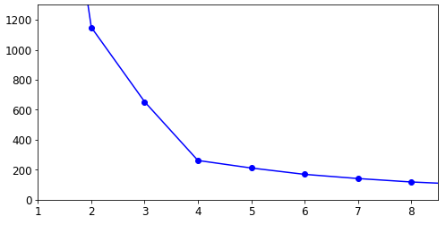
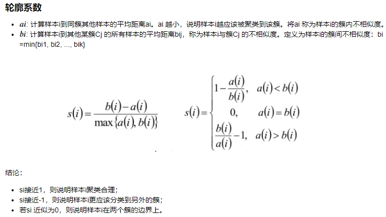
轮廓系数
另一种判断k值的 方法
python
from sklearn.metrics import silhouette_score
# 轮廓系数
silhouette_score(X,kmeans.labels_)
0.655517642572828

kmeans_per_k
[KMeans(algorithm='auto', copy_x=True, init='k-means++', max_iter=300,
     n_clusters=1, n_init=10, n_jobs=None, precompute_distances='auto',
     random_state=None, tol=0.0001, verbose=0),
 KMeans(algorithm='auto', copy_x=True, init='k-means++', max_iter=300,
     n_clusters=2, n_init=10, n_jobs=None, precompute_distances='auto',
     random_state=None, tol=0.0001, verbose=0)

silhouette_scores = [silhouette_score(X,model.labels_) for model in kmeans_per_k[1:]]
# 轮廓系数越接近1 说明越合理  但不一定最合理 只是参考
plt.figure(figsize=(8,4))
plt.plot(range(2,10),silhouette_scores,'bo-')
plt.show()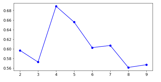
Kmeans存在的问题
python
# 评估只能当做参考
X1, y1 = make_blobs(n_samples=1000, centers=((4, -4), (0, 0)), random_state=42)
X1 = X1.dot(np.array([[0.374, 0.95], [0.732, 0.598]]))
X2, y2 = make_blobs(n_samples=250, centers=1, random_state=42)
X2 = X2 + [6, -8]
X = np.r_[X1, X2]
y = np.r_[y1, y2]

plot_data(X)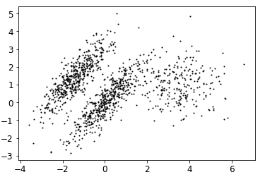
python
# 玩赖的 初始值规定了比较合理三个中心
# 事实上 即使inertia比较小 看出来分类也比较不合理
kmeans_good = KMeans(n_clusters=3,init=np.array([[-1.5,2.5],[0.5,0],[4,0]]),n_init=1,random_state=42)
kmeans_bad = KMeans(n_clusters=3,random_state=42)
kmeans_good.fit(X)
kmeans_bad.fit(X)

plt.figure(figsize = (10,4))
plt.subplot(121)
plot_decision_boundaries(kmeans_good,X)
plt.title('Good - inertia = {}'.format(kmeans_good.inertia_))

plt.subplot(122)
plot_decision_boundaries(kmeans_bad,X)
plt.title('Bad - inertia = {}'.format(kmeans_bad.inertia_))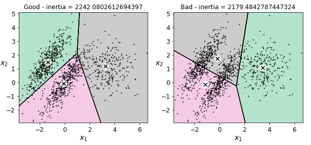
图像分割小例子
python
#ladybug.png 把向日葵从图像中分割出来
from matplotlib.image import imread
image = imread('ladybug.png')
image.shape
(533, 800, 3)


X = image.reshape(-1,3)
X.shape
(426400, 3)

kmeans = KMeans(n_clusters = 8,random_state=42).fit(X)
# 拿到中心位置
kmeans.cluster_centers_

# 需要还原成三维  图片
segmented_img = kmeans.cluster_centers_[kmeans.labels_].reshape(533, 800, 3)

segmented_imgs = []
n_colors = (10,8,6,4,2)
# 不同聚类中心进行展示
for n_cluster in n_colors:
    kmeans = KMeans(n_clusters = n_cluster,random_state=42).fit(X)
    segmented_img = kmeans.cluster_centers_[kmeans.labels_]
    segmented_imgs.append(segmented_img.reshape(image.shape))

plt.figure(figsize=(10,5))
plt.subplot(231)
plt.imshow(image)
plt.title('Original image')

for idx,n_clusters in enumerate(n_colors):
    plt.subplot(232+idx)
    plt.imshow(segmented_imgs[idx])
    plt.title('{}colors'.format(n_clusters))
半监督学习
用逻辑回归识别手写体数字,可以用无监督聚类提高准确率
python
# 首先,让我们将训练集聚类为50个集群, 然后对于每个聚类,让我们找到最靠近质心的图像。 我们将这些图像称为代表性图像
from sklearn.datasets import load_digits

X_digits,y_digits = load_digits(return_X_y = True)

from sklearn.model_selection import train_test_split

X_train,X_test,y_train,y_test = train_test_split(X_digits,y_digits,random_state=42)
# 有1347个手写体,8*8的像素点
X_train.shape
(1347, 64)
y_train.shape
(1347,)
python
#直接用逻辑回归的话 一般
#训练集只选了前50个
from sklearn.linear_model import LogisticRegression
n_labeled = 50

log_reg = LogisticRegression(random_state=42)
log_reg.fit(X_train[:n_labeled], y_train[:n_labeled])
log_reg.score(X_test, y_test)
0.8266666666666667

# 对这前50个进行聚类
k = 50
kmeans = KMeans(n_clusters=k, random_state=42)
X_digits_dist = kmeans.fit_transform(X_train)
X_digits_dist.shape
(1347, 50)
# 它用于返回数组中最小元素的索引
representative_digits_idx = np.argmin(X_digits_dist,axis=0)
representative_digits_idx.shape
(50,)

X_representative_digits = X_train[representative_digits_idx]

# 现在让我们绘制这些代表性图像并手动标记它们:
plt.figure(figsize=(8, 2))
for index, X_representative_digit in enumerate(X_representative_digits):
    plt.subplot(k // 10, 10, index + 1)
    plt.imshow(X_representative_digit.reshape(8, 8), cmap="binary", interpolation="bilinear")
    plt.axis('off')

plt.show()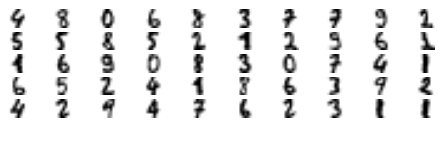
python
y_representative_digits = np.array([
    4, 8, 0, 6, 8, 3, 7, 7, 9, 2,
    5, 5, 8, 5, 2, 1, 2, 9, 6, 1,
    1, 6, 9, 0, 8, 3, 0, 7, 4, 1,
    6, 5, 2, 4, 1, 8, 6, 3, 9, 2,
    4, 2, 9, 4, 7, 6, 2, 3, 1, 1])
# 现在我们有一个只有50个标记实例的数据集,它们中的每一个都是其集群的代表性图像,而不是完全随机的实例。 让我们看看性能是否更好:

log_reg = LogisticRegression(random_state=42)
log_reg.fit(X_representative_digits, y_representative_digits)
log_reg.score(X_test, y_test)
0.9244444444444444
python
# 但也许我们可以更进一步:如果我们将标签传播到同一群集中的所有其他实例,该怎么办?
y_train_propagated = np.empty(len(X_train), dtype=np.int32)
for i in range(k):
    y_train_propagated[kmeans.labels_==i] = y_representative_digits[i]

log_reg = LogisticRegression(random_state=42)
log_reg.fit(X_train, y_train_propagated)
LogisticRegression(C=1.0, class_weight=None, dual=False, fit_intercept=True,
          intercept_scaling=1, max_iter=100, multi_class='warn',
          n_jobs=None, penalty='l2', random_state=42, solver='warn',
          tol=0.0001, verbose=0, warm_start=False)

log_reg.score(X_test, y_test)
0.9288888888888889
python
#只选择前20个来试试
percentile_closest = 20

X_cluster_dist = X_digits_dist[np.arange(len(X_train)), kmeans.labels_]
for i in range(k):
    in_cluster = (kmeans.labels_ == i)
    cluster_dist = X_cluster_dist[in_cluster] #选择属于当前簇的所有样本
    cutoff_distance = np.percentile(cluster_dist, percentile_closest) #排序找到前20个
    above_cutoff = (X_cluster_dist > cutoff_distance) # False True结果
    X_cluster_dist[in_cluster & above_cutoff] = -1

partially_propagated = (X_cluster_dist != -1)
X_train_partially_propagated = X_train[partially_propagated]
y_train_partially_propagated = y_train_propagated[partially_propagated]

log_reg = LogisticRegression(random_state=42)
log_reg.fit(X_train_partially_propagated, y_train_partially_propagated)

log_reg.score(X_test, y_test)
0.9422222222222222
DBSCAN
python
from sklearn.datasets import make_moons
X, y = make_moons(n_samples=1000, noise=0.05, random_state=42)

plt.plot(X[:,0],X[:,1],'b.')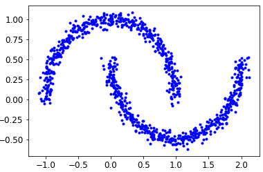
python
from sklearn.cluster import DBSCAN
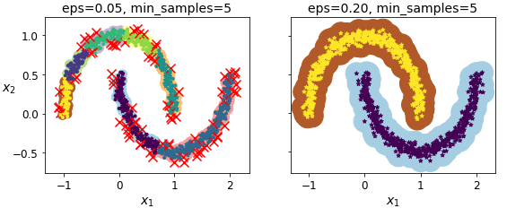
dbscan = DBSCAN(eps = 0.05,min_samples=5)
dbscan.fit(X)
DBSCAN(algorithm='auto', eps=0.05, leaf_size=30, metric='euclidean',
    metric_params=None, min_samples=5, n_jobs=None, p=None)


dbscan.labels_[:10]
array([ 0,  2, -1, -1,  1,  0,  0,  0,  2,  5], dtype=int64)
dbscan.core_sample_indices_[:10]
array([ 0,  4,  5,  6,  7,  8, 10, 11, 12, 13], dtype=int64)
np.unique(dbscan.labels_) #相当于看集合了
array([-1,  0,  1,  2,  3,  4,  5,  6], dtype=int64)

dbscan2 = DBSCAN(eps = 0.2,min_samples=5)
dbscan2.fit(X)
DBSCAN(algorithm='auto', eps=0.2, leaf_size=30, metric='euclidean',
    metric_params=None, min_samples=5, n_jobs=None, p=None)
python
def plot_dbscan(dbscan, X, size, show_xlabels=True, show_ylabels=True):
    core_mask = np.zeros_like(dbscan.labels_, dtype=bool)
    core_mask[dbscan.core_sample_indices_] = True
    anomalies_mask = dbscan.labels_ == -1
    non_core_mask = ~(core_mask | anomalies_mask)

    cores = dbscan.components_
    anomalies = X[anomalies_mask]
    non_cores = X[non_core_mask]

    plt.scatter(cores[:, 0], cores[:, 1],
                c=dbscan.labels_[core_mask], marker='o', s=size, cmap="Paired")
    plt.scatter(cores[:, 0], cores[:, 1], marker='*', s=20, c=dbscan.labels_[core_mask])
    plt.scatter(anomalies[:, 0], anomalies[:, 1],
                c="r", marker="x", s=100)
    plt.scatter(non_cores[:, 0], non_cores[:, 1], c=dbscan.labels_[non_core_mask], marker=".")
    if show_xlabels:
        plt.xlabel("$x_1$", fontsize=14)
    else:
        plt.tick_params(labelbottom='off')
    if show_ylabels:
        plt.ylabel("$x_2$", fontsize=14, rotation=0)
    else:
        plt.tick_params(labelleft='off')
    plt.title("eps={:.2f}, min_samples={}".format(dbscan.eps, dbscan.min_samples), fontsize=14)

plt.figure(figsize=(9, 3.2))

plt.subplot(121)
plot_dbscan(dbscan, X, size=100)

plt.subplot(122)
plot_dbscan(dbscan2, X, size=600, show_ylabels=False)
plt.show()