 阿源的知识库
降维
26. 线性判别分析降维 LDA
python
# 适用于有监督 分类 的数据初始降维
# 必须是有监督问题
feature_dict = {i:label for i,label in zip(
                range(4),
                  ('sepal length in cm',
                  'sepal width in cm',
                  'petal length in cm',
                  'petal width in cm', ))}

import pandas as pd

df = pd.io.parsers.read_csv(
    filepath_or_buffer='https://archive.ics.uci.edu/ml/machine-learning-databases/iris/iris.data',
    header=None,
    sep=',',
    )
df.columns = [l for i,l in sorted(feature_dict.items())] + ['class label']
df.dropna(how="all", inplace=True) # to drop the empty line at file-end

df.tail()
sepal length in cm	sepal width in cm	petal length in cm	petal width in cm	class label
145	6.7	3.0	5.2	2.3	Iris-virginica
146	6.3	2.5	5.0	1.9	Iris-virginica

from sklearn.preprocessing import LabelEncoder

X = df[['sepal length in cm','sepal width in cm','petal length in cm','petal width in cm']].values
y = df['class label'].values

# 把标签变成数字快捷写法
enc = LabelEncoder()
label_encoder = enc.fit(y)
y = label_encoder.transform(y) + 1

#label_dict = {1: 'Setosa', 2: 'Versicolor', 3:'Virginica'}
python
import numpy as np
np.set_printoptions(precision=4)

mean_vectors = []
for cl in range(1,4):
    mean_vectors.append(np.mean(X[y==cl], axis=0))
    print('Mean Vector class %s: %s\n' %(cl, mean_vectors[cl-1]))


Mean Vector class 1: [ 5.006  3.418  1.464  0.244]
Mean Vector class 2: [ 5.936  2.77   4.26   1.326]
Mean Vector class 3: [ 6.588  2.974  5.552  2.026]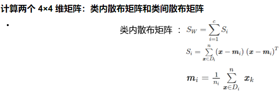
python
S_W = np.zeros((4,4))
for cl,mv in zip(range(1,4), mean_vectors):
    class_sc_mat = np.zeros((4,4))                  # scatter matrix for every class
    for row in X[y == cl]:
        row, mv = row.reshape(4,1), mv.reshape(4,1) # make column vectors
        class_sc_mat += (row-mv).dot((row-mv).T)
    S_W += class_sc_mat                             # sum class scatter matrices
print('within-class Scatter Matrix:\n', S_W)
python
overall_mean = np.mean(X, axis=0)

S_B = np.zeros((4,4))
for i,mean_vec in enumerate(mean_vectors):
    n = X[y==i+1,:].shape[0]
    mean_vec = mean_vec.reshape(4,1) # make column vector
    overall_mean = overall_mean.reshape(4,1) # make column vector
    S_B += n * (mean_vec - overall_mean).dot((mean_vec - overall_mean).T)

print('between-class Scatter Matrix:\n', S_B)
python
eig_vals, eig_vecs = np.linalg.eig(np.linalg.inv(S_W).dot(S_B))
# 算每个特征的特征值和特征向量
for i in range(len(eig_vals)):
    eigvec_sc = eig_vecs[:,i].reshape(4,1)
    print('\nEigenvector {}: \n{}'.format(i+1, eigvec_sc.real))
    print('Eigenvalue {:}: {:.2e}'.format(i+1, eig_vals[i].real))
python
#特征向量:表示映射方向
#特征值:特征向量的重要程度
#Make a list of (eigenvalue, eigenvector) tuples
eig_pairs = [(np.abs(eig_vals[i]), eig_vecs[:,i]) for i in range(len(eig_vals))]
# Sort the (eigenvalue, eigenvector) tuples from high to low
eig_pairs = sorted(eig_pairs, key=lambda k: k[0], reverse=True)
# Visually confirm that the list is correctly sorted by decreasing eigenvalues
print('Eigenvalues in decreasing order:\n')
for i in eig_pairs:
    print(i[0])
Eigenvalues in decreasing order:
32.2719577997
0.27756686384
7.7995841654e-15
5.76433252705e-15

print('Variance explained:\n')
eigv_sum = sum(eig_vals)
for i,j in enumerate(eig_pairs):
    print('eigenvalue {0:}: {1:.2%}'.format(i+1, (j[0]/eigv_sum).real))
Variance explained:

eigenvalue 1: 99.15%
eigenvalue 2: 0.85%
eigenvalue 3: 0.00%
eigenvalue 4: 0.00%
python
# 选择前两维特征
W = np.hstack((eig_pairs[0][1].reshape(4,1), eig_pairs[1][1].reshape(4,1)))
print('Matrix W:\n', W.real)
Matrix W:
 [[ 0.2049 -0.009 ]
 [ 0.3871 -0.589 ]
 [-0.5465  0.2543]
 [-0.7138 -0.767 ]]
X_lda = X.dot(W)
assert X_lda.shape == (150,2), "The matrix is not 150x2 dimensional."
python
from matplotlib import pyplot as plt

def plot_step_lda():

    ax = plt.subplot(111)
    for label,marker,color in zip(
        range(1,4),('^', 's', 'o'),('blue', 'red', 'green')):

        plt.scatter(x=X_lda[:,0].real[y == label],
                y=X_lda[:,1].real[y == label],
                marker=marker,
                color=color,
                alpha=0.5,
                label=label_dict[label]
                )

    plt.xlabel('LD1')
    plt.ylabel('LD2')

    leg = plt.legend(loc='upper right', fancybox=True)
    leg.get_frame().set_alpha(0.5)
    plt.title('LDA: Iris projection onto the first 2 linear discriminants')

    # hide axis ticks
    plt.tick_params(axis="both", which="both", bottom="off", top="off",
            labelbottom="on", left="off", right="off", labelleft="on")

    # remove axis spines
    ax.spines["top"].set_visible(False)
    ax.spines["right"].set_visible(False)
    ax.spines["bottom"].set_visible(False)
    ax.spines["left"].set_visible(False)

    plt.grid()
    plt.tight_layout
    plt.show()

plot_step_lda()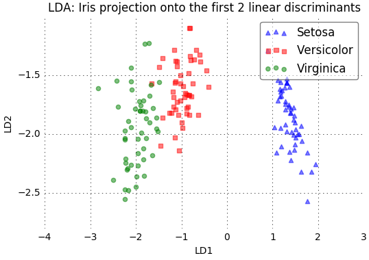
官方的包
python
from sklearn.discriminant_analysis import LinearDiscriminantAnalysis as LDA

# LDA
sklearn_lda = LDA(n_components=2)
X_lda_sklearn = sklearn_lda.fit_transform(X, y)

def plot_scikit_lda(X, title):

    ax = plt.subplot(111)
    for label,marker,color in zip(
        range(1,4),('^', 's', 'o'),('blue', 'red', 'green')):

        plt.scatter(x=X[:,0][y == label],
                    y=X[:,1][y == label] * -1, # flip the figure
                    marker=marker,
                    color=color,
                    alpha=0.5,
                    label=label_dict[label])

    plt.xlabel('LD1')
    plt.ylabel('LD2')

    leg = plt.legend(loc='upper right', fancybox=True)
    leg.get_frame().set_alpha(0.5)
    plt.title(title)

    # hide axis ticks
    plt.tick_params(axis="both", which="both", bottom="off", top="off",
            labelbottom="on", left="off", right="off", labelleft="on")

    # remove axis spines
    ax.spines["top"].set_visible(False)
    ax.spines["right"].set_visible(False)
    ax.spines["bottom"].set_visible(False)
    ax.spines["left"].set_visible(False)

    plt.grid()
    plt.tight_layout
    plt.show()

plot_step_lda()
plot_scikit_lda(X_lda_sklearn, title='Default LDA via scikit-learn')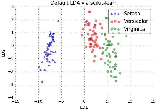
27.主成分分析降维 PCA
python
# 无监督 的  可以降维
import numpy as np
import pandas as pd
df = pd.read_csv('iris.data')
df.head()
df.columns=['sepal_len', 'sepal_wid', 'petal_len', 'petal_wid', 'class']
df.head()
sepal_len	sepal_wid	petal_len	petal_wid	class
0	4.9	3.0	1.4	0.2	Iris-setosa
1	4.7	3.2	1.3	0.2	Iris-setosa
2	4.6	3.1	1.5	0.2	Iris-setos
python
# split data table into data X and class labels y
X = df.ix[:,0:4].values
y = df.ix[:,4].values

from matplotlib import pyplot as plt
import math

label_dict = {1: 'Iris-Setosa',
              2: 'Iris-Versicolor',
              3: 'Iris-Virgnica'}

feature_dict = {0: 'sepal length [cm]',
                1: 'sepal width [cm]',
                2: 'petal length [cm]',
                3: 'petal width [cm]'}


plt.figure(figsize=(8, 6))
for cnt in range(4):
    plt.subplot(2, 2, cnt+1)
    for lab in ('Iris-setosa', 'Iris-versicolor', 'Iris-virginica'):
        plt.hist(X[y==lab, cnt],
                     label=lab,
                     bins=10,
                     alpha=0.3,)
    plt.xlabel(feature_dict[cnt])
    plt.legend(loc='upper right', fancybox=True, fontsize=8)

plt.tight_layout()
plt.show()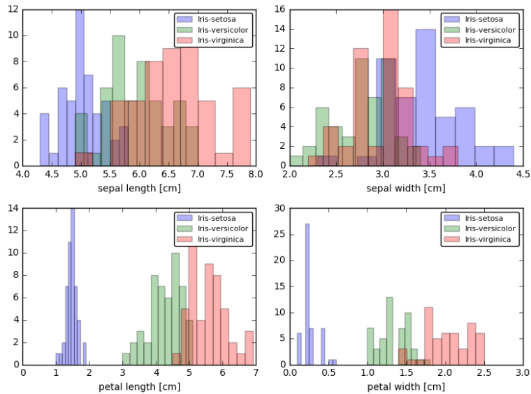
python
from sklearn.preprocessing import StandardScaler
X_std = StandardScaler().fit_transform(X)
mean_vec = np.mean(X_std, axis=0)
cov_mat = (X_std - mean_vec).T.dot((X_std - mean_vec)) / (X_std.shape[0]-1)
print('Covariance matrix \n%s' %cov_mat)
print('NumPy covariance matrix: \n%s' %np.cov(X_std.T))

cov_mat = np.cov(X_std.T)
# 来计算给定矩阵cov_mat的特征值和特征向量
eig_vals, eig_vecs = np.linalg.eig(cov_mat)
print('Eigenvectors \n%s' %eig_vecs)
print('\nEigenvalues \n%s' %eig_vals)
Eigenvectors
[[ 0.52308496 -0.36956962 -0.72154279  0.26301409]
 [-0.25956935 -0.92681168  0.2411952  -0.12437342]
 [ 0.58184289 -0.01912775  0.13962963 -0.80099722]
 [ 0.56609604 -0.06381646  0.63380158  0.52321917]]

Eigenvalues
[ 2.92442837  0.93215233  0.14946373  0.02098259]

# Make a list of (eigenvalue, eigenvector) tuples
eig_pairs = [(np.abs(eig_vals[i]), eig_vecs[:,i]) for i in range(len(eig_vals))]
print (eig_pairs)
print ('----------')
# Sort the (eigenvalue, eigenvector) tuples from high to low
eig_pairs.sort(key=lambda x: x[0], reverse=True)
# Visually confirm that the list is correctly sorted by decreasing eigenvalues
print('Eigenvalues in descending order:')
for i in eig_pairs:
    print(i[0])

tot = sum(eig_vals)
var_exp = [(i / tot)*100 for i in sorted(eig_vals, reverse=True)]
print (var_exp)
# 计算输入数组的累积和
cum_var_exp = np.cumsum(var_exp)
cum_var_exp
[72.620033326920336, 23.147406858644135, 3.7115155645845164, 0.52104424985101538]
array([  72.62003333,   95.76744019,   99.47895575,  100.        ])

plt.figure(figsize=(6, 4))

plt.bar(range(4), var_exp, alpha=0.5, align='center',
            label='individual explained variance')
plt.step(range(4), cum_var_exp, where='mid',
             label='cumulative explained variance')
plt.ylabel('Explained variance ratio')
plt.xlabel('Principal components')
plt.legend(loc='best')
plt.tight_layout()
plt.show()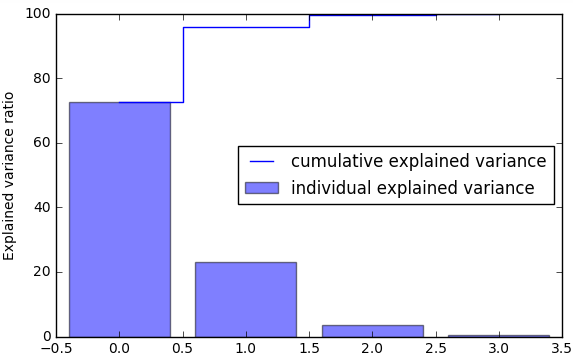
python
matrix_w = np.hstack((eig_pairs[0][1].reshape(4,1),
                      eig_pairs[1][1].reshape(4,1)))

print('Matrix W:\n', matrix_w)

Y = X_std.dot(matrix_w)  # 降维后的数据
array([[-2.10795032,  0.64427554],
       [-2.38797131,  0.30583307],
python
plt.figure(figsize=(6, 4))
for lab, col in zip(('Iris-setosa', 'Iris-versicolor', 'Iris-virginica'),
                        ('blue', 'red', 'green')):
     plt.scatter(X[y==lab, 0],
                X[y==lab, 1],
                label=lab,
                c=col)
plt.xlabel('sepal_len')
plt.ylabel('sepal_wid')
plt.legend(loc='best')
plt.tight_layout()
plt.show()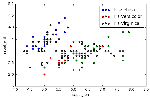
python
plt.figure(figsize=(6, 4))
for lab, col in zip(('Iris-setosa', 'Iris-versicolor', 'Iris-virginica'),
                        ('blue', 'red', 'green')):
     plt.scatter(Y[y==lab, 0],
                Y[y==lab, 1],
                label=lab,
                c=col)
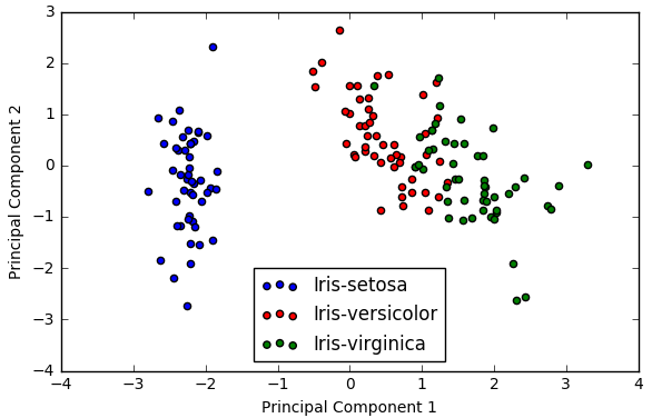
plt.xlabel('Principal Component 1')
plt.ylabel('Principal Component 2')
plt.legend(loc='lower center')
plt.tight_layout()
plt.show()