 阿源的知识库
支持向量机
16. 支持向量机原理
17. 支持向量机实验分析
python
# 与传统算法进行对比,看看SVM究竟能带来什么样的效果
# 软间隔的作用,这么复杂的算法肯定会导致过拟合现象,如何来进行解决呢?
# 核函数的作用,如果只是做线性分类,好像轮不到SVM登场了,核函数才是它的强大之处!
import numpy as np
import os
%matplotlib inline
import matplotlib
import matplotlib.pyplot as plt
plt.rcParams['axes.labelsize'] = 14
plt.rcParams['xtick.labelsize'] = 12
plt.rcParams['ytick.labelsize'] = 12
import warnings
warnings.filterwarnings('ignore')
支持向量机带来的效果
python
from sklearn.svm import SVC
from sklearn import datasets

iris = datasets.load_iris()
X = iris['data'][:,(2,3)]
y = iris['target']

setosa_or_versicolor = (y==0)|(y==1)
X = X[setosa_or_versicolor]
y = y[setosa_or_versicolor]

svm_clf = SVC(kernel='linear',C=float('inf'))
svm_clf.fit(X,y)
SVC(C=inf, cache_size=200, class_weight=None, coef0=0.0,
  decision_function_shape='ovr', degree=3, gamma='auto_deprecated',
  kernel='linear', max_iter=-1, probability=False, random_state=None,
  shrinking=True, tol=0.001, verbose=False)
python
# 一般的模型
x0 = np.linspace(0, 5.5, 200)
pred_1 = 5*x0 - 20
pred_2 = x0 - 1.8
pred_3 = 0.1 * x0 + 0.5

def plot_svc_decision_boundary(svm_clf, xmin, xmax,sv=True):
    w = svm_clf.coef_[0]
    b = svm_clf.intercept_[0]
    print (w)
    x0 = np.linspace(xmin, xmax, 200)
    decision_boundary = - w[0]/w[1] * x0 - b/w[1]
    margin = 1/w[1]
    gutter_up = decision_boundary + margin
    gutter_down = decision_boundary - margin
    if sv:
        svs = svm_clf.support_vectors_
        plt.scatter(svs[:,0],svs[:,1],s=180,facecolors='#FFAAAA')
    plt.plot(x0,decision_boundary,'k-',linewidth=2)
    plt.plot(x0,gutter_up,'k--',linewidth=2)
    plt.plot(x0,gutter_down,'k--',linewidth=2)
plt.figure(figsize=(14,4))
plt.subplot(121)
plt.plot(X[:,0][y==1],X[:,1][y==1],'bs')
plt.plot(X[:,0][y==0],X[:,1][y==0],'ys')
plt.plot(x0,pred_1,'g--',linewidth=2)
plt.plot(x0,pred_2,'m-',linewidth=2)
plt.plot(x0,pred_3,'r-',linewidth=2)
plt.axis([0,5.5,0,2])

plt.subplot(122)
plot_svc_decision_boundary(svm_clf, 0, 5.5)
plt.plot(X[:,0][y==1],X[:,1][y==1],'bs')
plt.plot(X[:,0][y==0],X[:,1][y==0],'ys')
plt.axis([0,5.5,0,2])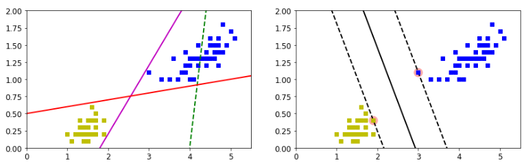
数据标准化的影响